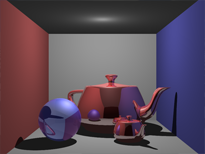
CS 6620, Advanced Computer Graphics II
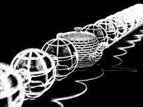
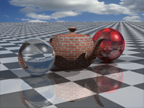
During this class, we started with ray casting, then progressed towards Monte Carlo Ray Tracing and Photon Maping. I sat in on it and was able to complete only part of the work (9 of 12 projects), see (class page), which can be seen in the link below.
Projects
- setting up
- ray casting (visibility)
- shading
- shadows, reflections and refractions
- triangular meshes
- space partitioning
- textures
- antialiasing
- depth of field
- soft shadows and glossy surfaces
Project 9: Soft shadows and glossy surfaces
Updated: 11.06.12
Description
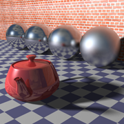
The main part of this project is to implement soft shadows and glossy reflections. There were a few optional features: glossy refractions, use importance sampling for glossy reflections/refractions, implement area lights for shading, use Quasi Monte-Carlo sequence for all features above.
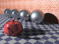
I was able to make time to generate the required image showing glossy reflections and soft shadows.
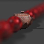
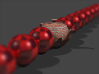
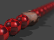
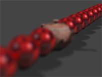
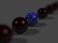
The circular lens/aperture is being sampled using equal area weighting with the two random variables being selected using Halton sequence base 2 and 3. Here are some images of the results when using 64 and 300 samples per pixel. The rendering times were 4.81 sec (3.66 sec) and 10.52 sec (8.0 sec) when using 4 (8) threads.
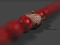
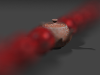
When looking at different aperture sizes, we get the following images (rendered with 1000 spp), from left to right we have aperture radii of 1.5, 6 and 10.
Messing around with the depth of field, we can focus on various objects in the scene. From left to right, we have depths of 50, 80, and 110.
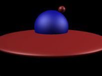
A final fun image is shown below
Project 7: Antialiasing
Updated: 10.29.12
Description
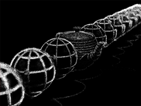
We were to implement adaptive antialiasing with multiple samples per pixel, render one or more scenes using antialiasing, and generate an image that shows the number of samples per pixel as pixel intensity. An optional feature was to implement reconstruction filtering.
I've implemented pixel sampling using Halton Sequence base 5 for x-dimension and 7 for y-dimension. The adaptive sampler allows to set minimum and maximum number of samples per pixel and an error tolerance (in L infinity norm).
The top row of the images below use no ray differentials. The bottom row uses ray differentials with 16 samples per texture lookup. from left to right, the images are organized have 4, 16, and 64 samples per pixel.
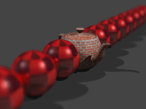
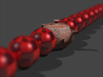
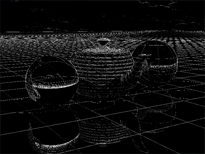
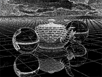
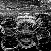
Now, using the adaptive pixel color tolerance, we can generate the following images. Top row is the rendered image, while bottom row shows the pixel errors. From left to right: 16 spt, 16 spp, and 0.03 tol; 64 spt, 64 spp, and 0.003 tol; no ray differentials, 16 spp, and 0.03 tol.
The rendering times using 64 spt and 64 spp changed from 113,000 sec (81,500 sec) to 9,520 sec (6,790 sec) when using adaptive rendered with tolerance of 0.03 (times are for 4 and 8 cores respectively).
Project 6: Textures
Updated: 10.27.12
Description
We were to implement a procedural checker-board texture, load PPM image files and use them as textures, use an image as background, use an image as reflection/refraction environment, compute texture coordinates for all objects (sphere, plane, and triangular mesh), compute texture coordinate derivatives using ray differentials.
The additional features were: implement MIP mapping and anisotropic filtering for efficient texture filtering.
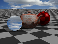
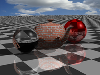
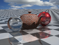
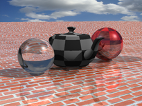
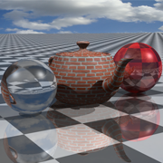
Below are a few of the few images which show off the features described above. The left-most image shows model texturing via checkerboard and images, as well as an image for background (when a ray doesn't hit anything). The middle image adds reflections and refractions. The right-most image shows using the cloud image for reflection/refraction environment mapping (using spherical coordinates).
Now, the ray differentials have been implemented following the basic path given in pbrt 2. There are two additional rays kept in the data structure which maintain the footprint of the pixel. The idea is to keep track of differential geometry (essentially parameterizing the local tangent plane) at every intersection and then use it to compute ray differentials once the closest hit has been generated. Another approach is to intersect that plane with differential rays and compute the ray differentials per intersection.
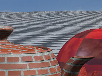
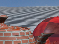
My raytracer has been extended to turn ray differentials and mip-mapping on/off, as well as selecting the number of samples to use for texture anti-aliasing when using ray differentials. The images below show the images as the number of samples increases from 4, to 16, to 64. Top row shows random sampling, while the bottom row shows Halton sequence base 2 for u and Halton sequence base 3 for v texture coordinates.
It's great to see that Halton sequences work rather well even at a modest number of texture samples of 16, while the random sampler has a significant amount of noise. However at 64 texture samples per pixels, the two techniques are almost similar.
I've also added ray differential computations for reflections and refractions. However, it seems that using a simple planar approximation for refractions on a sphere isn't god enough - the checkerboard is a bit fuzzy on the top fo the refractive sphere, as well as the reflection of the pattern through the sphere. A way to fix it would be keeping track of the partial derivatives of the normal vector wrt world coordinates.
I've also implemented isotropic mipmaps, which use trilinear interpolation between 8 image samples (4 per mipmap level). Below are images for comparison: left - no mip-maps or ray differentials, middle - no mip-maps with ray differentials, right - both mip maps and ray differentials. One can see that mip-maps do fairly well with texture sampling in terms of noise, but they aren't perfect when compared to ray-differentials because they don't handle anisotropy well. One can extend mip-maps to be anisotropic. Of course, mip-maps cost 1/8th the number of samples per texture map lookup!
Here are final render times for a few the required image using 4 and 8 cores (in brackets). The triangle mesh uses a KD-tree for acceleration.
- ray differentials, 64 spt: 1.985 sec (1.386 sec)
- ray differentials, no refraction, 64 spt: 1.914 sec (1.376 sec)
- no ray differentials: 0.801 sec (0.634 sec)
Final scene:
- mip-maps, ray differentials, 8 spt: 1.190 sec (0.856 sec)
- ray differentials, 64 spt: 2.023 sec (1.455 sec)
- ray-differentials, 8 spt: 0.933 sec (0.723 sec)
- nothing: 0.802 sec (0.617 sec)
Project 5: Space partitioning
Updated: 10.01.12
Description
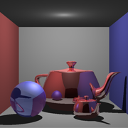
We were to implement building BVH for all triangular mesh objects in the scene, use the BVH to avoid unnecessary triangle intersection computation, and report render times with and without BVH. Additions: use BVH for the node structure as well, implement different ways of building the BVH tree (such as using median splitting or surface area heuristics) and compare the results, mplement kd-tree as an alternative to BVH.
I wanted to check out how the rendering times differ between different number of parallel threads, using GUI and bounding boxes. Each of the images was rendered using Intel i7-2600K processor running at 3.4 GHz, rendering 64x64 image tiles. Based on the last assignment it doesn't make much difference between GUI and CMD runtimes, so I'll use GUI here.
So let's start with the timing table measured in seconds.
| Render threads: | 1 | 2 | 3 | 4 | 6 | 8 |
|---|---|---|---|---|---|---|
| Brute force | 328.562 | 166.213 | 119.282 | 94.413 | 76.743 | 66.364 |
| Bounding boxes | 53.602 | 27.288 | 19.186 | 15.598 | 12.312 | 11.142 |
| BVH | 1.302 | 0.673 | 0.488 | 0.402 | 0.340 | 0.332 |
Then, we can look at the speedup over brute force depending on which acceleration structure we use. On average, bounding boxes per scene node provide about 6.1x, BVH (built top down, dividing each box in half) provides about 234.1x speedups.
| Render threads: | 1 | 2 | 3 | 4 | 6 | 8 | Ave |
|---|---|---|---|---|---|---|---|
| Bounding Boxes | 6.130 | 6.091 | 6.217 | 6.053 | 6.233 | 5.956 | 6.113 |
| BVH | 252.438 | 247.014 | 244.521 | 234.989 | 225.788 | 199.893 | 234.107 |

Project 4: Triangular meshes
Updated: 09.24.12
Description
We were to implement plane, triangle, and bounding box intersections. Then render a scene which had a refractive sphere and two instances of a reflective teapot. In addition, we needded to compare render times when (not) using bounding boxes to test intersections for objects and scene nodes. All of the renderings were limited to 10 ray bounces, which is a bit of an overkill in our scene.
I wanted to check out how the rendering times differ between different number of parallel threads, using GUI and bounding boxes. Each of the images was rendered using Intel i7-2600K processor running at 3.4 GHz, rendering 64x64 image tiles.
So let's start with the timing table measured in seconds.
| Render threads: | 1 | 2 | 3 | 4 | 6 | 8 |
|---|---|---|---|---|---|---|
| GUI | 328.562 | 166.213 | 119.282 | 94.413 | 76.743 | 66.364 |
| CMD | 327.726 | 166.41 | 119.223 | 93.898 | 76.544 | 66.410 |
| GUI, boxes | 53.602 | 27.288 | 19.186 | 15.598 | 12.312 | 11.142 |
| CMD, boxes | 53.357 | 27.212 | 19.150 | 15.071 | 12.252 | 11.049 |
Now we can look at the scaling in relation to the number of threads being used. It's interesting to note that the scaling is almost linear up to 4 threads, which makes sense because this is a quad-core processor. We get into diminishing returns once we start utilizing the Hyper-threaded cores (but there's still an overall speed-up). Another reason for this is that the tile size chosen is too large and doesn't result in great load balancing (this is obvious when looking at the rendering in the GUI mode, because one tile finishes a lot later).
| Render threads: | 1 | 2 | 3 | 4 | 6 | 8 |
|---|---|---|---|---|---|---|
| GUI | 1 | 1.977 | 2.754 | 3.480 | 4.281 | 4.951 |
| CMD | 1 | 1.969 | 2.749 | 3.490 | 4.282 | 4.935 |
| GUI, boxes | 1 | 1.964 | 2.794 | 3.436 | 4.354 | 4.811 |
| CMD, boxes | 1 | 1.961 | 2.786 | 3.540 | 4.355 | 4.829 |
| Ave | 1 | 1.968 | 2.771 | 3.487 | 4.318 | 4.881 |
Finally, we can look at the speedup when using bounding boxes. On average, they provide about 6.15x.
| Render threads: | 1 | 2 | 3 | 4 | 6 | 8 | Ave |
|---|---|---|---|---|---|---|---|
| GUI | 6.130 | 6.091 | 6.217 | 6.053 | 6.233 | 5.956 | 6.113 |
| CMD | 6.142 | 6.115 | 6.226 | 6.230 | 6.247 | 6.011 | 6.162 |
| Ave | 6.136 | 6.103 | 6.222 | 6.142 | 6.240 | 5.983 | 6.138 |
Here are a few interesting images that I rendered. The left-most is an interesting bug, which was induced by a slightly wrong sphere intersection test. The middle image shows the box intersection test on scene 2, and the right image shows the box intersection test for the scene 4.
The left image is the required image (4k x 3k resolution), but the right image has the larger teapot as a dark glass material (4k x 3k resolution).
Project 3: Shadows, reflections and refractions
Updated: 09.15.12
Description
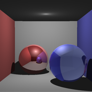
We were required to add shadows, reflections and refractions to our ray tracer. The material we're using is still Blinn-Phong therefore the reflections have a strong diffuse/specular component. There is also an update to include reflection and refraction coefficients (colors) to add some complexity on top of Blinn-Phong base shading. Also, the refractive materials have some absorption which is taken into account based on the distance that a ray travels through.
In addition to all of the above, refractive objects use Schlick's approximation to compute Fresnel terms. I've also added a maximum ray depth for reflected/refracted rays. Also there was a need to introduce clamping final colors to (0,1) before writing it out to a framebuffer.
There are a whole bunch of images to show. First off are shadows and (perfect) reflection.
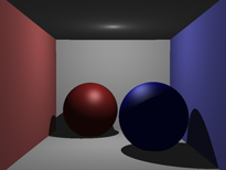
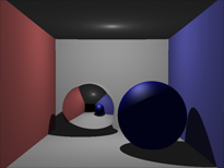
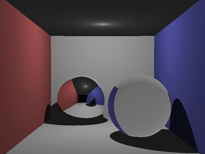
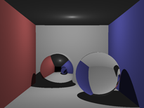
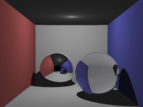
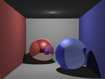
Below is a progression of images showing the implementation of refraction. The leftmost image shows refraction from the first interface. Then, complete refraction (accounting for the back of the right sphere). The rightmost image below shows the effect of Schlick approximation being used to combine reflection with refraction.
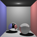
Finally, we can add absorption (left image). The middle image shows the final required rendering when all of the features have been turned on. The rightmost image shows a rendering of another Cornell Box (reference image).
Project 2: Shading
Updated: 09.08.12
Description
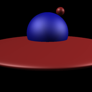
This project had several things to work on. I've added support for reading materials and lights from the scene file. There are several lights being supported: point, directional and ambient. The only material being supported is Blinn-Phong, and I didn't add any extras.
The software has been re-engineered somewhat to allow ease of replacing renderers. The GUI has been updated and both visibility and shadowless direct lighting can be used interchangeably. Also OpenGL renderer has been updated to show Phong shaded scenes.
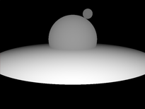
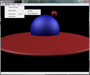
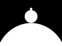
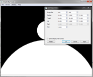
The images below show (left to right) shadowless direct illumination, depth buffer and UI screenshot with OpenGL renderer.
Project 1: Ray casting (visibility)
Updated: 09.04.12
Description
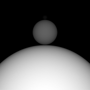
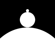
This project had several things to work on. Primarily, it was geared at ray-casting the scene with some spheres and displaying visibility. Also, I've added depth buffer output, as well as multi-threading. All of these were added to the base framework I wrote out for project setup.
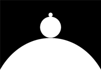
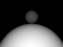
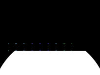
The images below show (left to right) visibility computed with ray casting, depth buffer and the multi-threaded computation (each tile with colored corners corresponds to a single thread).
Project 0: Setting up
Updated: 09.04.12
Description
This project was basically designed to parse an XML scene, build scene hierarchy and save rendered images. I've decided to build the entire framework from scratch in C++ using Qt 4.8. This took a little bit of extra time, but allows a lot of flexibility in terms of building up the GUI and interfacing with it easily. The framework allows for GUI and Command-line rendering, OpenGL display of scene, interactive camera modification and saving updated scenes.
The images below show the OpenGL output for the default scene as well as the basic UI (from left to right).
